Copyright (c) Susan Laflin. August 1999.

The references for this topic are :-
Rogers & Adams chapter 6 sections 6.8 & 6.9.
Faux & Pratt sections 7.1 & 7.3.

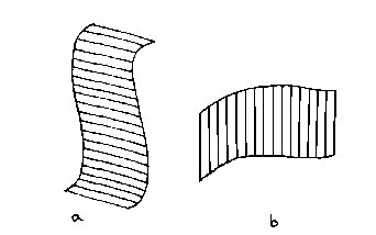
When we come to deal with ruled or lofted surfaces, we are dealing with surfaces where the curvature is very much greater in one direction. One example of such a surface could be an aircraft wing, where the cross-section is very curved but there is very little change in slope as you move along the wing from the aircraft body to the tip. Examples of lofted surfaces are shown in the figure below:

Lofted Surfaces

The case shown in diagram (a) uses linear interpolation parallel to the u or x-axis and a general edge-curve in the v-direction. This corresponds to the equation:

r(u,v) = (1-u)*r(0,v) + u*r(1,v)

where r(0,v) and r(1,v) are the two edge-curves. The other case, shown in diagram (b) uses linear interpolation in the v-direction and edge-curves in the u-direction. It corresponds to the equation:

r(u,v) = (1-v)*r(u,0) + v*r(u,1)

where r(u,0) and r(u,1) are the two edge curves.

When we wish to move to the full complexity of edge-curves in both directions, we have to move to one of the Coon's surfaces. The Bi-Cubic Surface Patch is one example of a Coons surface, but initially we shall look at the linear Coon's Surface. To develop this, we start by taking a linear combination of the four edge curves, giving:

(1-v)*r(u,0) + v*r(u,1) + (1-u)*r(0,v) + u*r(1,v)

This is effectively the sum of two Lofted surfaces and so it is no surprise to note that the values at the four corners are twice the amount required. This can be corrected by subtracting the corner values i.e.

(1-u)*(1-v)*r(0,0)+(1-u)*v*r(0,1)+u*(1-v)*r(1,0)+u*v*r(1,1)

Thus the equation of the linear Coons' surface, expressed in matrix form, becomes:

r(u,v) ={ (1-u), u , 1 ] -r(0,0)  -r(0,1)  r(0,v)	(1-v) 
                         -r(1,0)  -r(1,1)  r(1,v)	  v
                          r(u,0)   r(u,1)    0 		  1

This is expressed in terms of the "blending functions", the "edge curves" and the "values" at the corners. Since any two adjacent patches will meet along an edge curve, we can always choose these curves to be the same, so that r(u,0) for one patch has the same equation as r(u,1) for the other. This ensures that the overall surface has no holes in it. Since the blending curves are still linear, it is still not possible to ensure continuity of gradient as we move from one patch to the next.